🌳 Hierarchical selection function for a subset of the Gaia catalogue

last updated: 2024-06-13

The GaiaUnlimited module subsample provides a simple way of counting sources satisfying user-defined criteria, out of the whole Gaia catalogue. The result is given per bin of magnitude and/or colour, and per healpix region on the sky. The colour and magnitude binning can be chosen by the user, as well as the spatial resolution (order of the healpix tessellation).

Before going through this tutorial, the user is encouraged to familiarise themselves with the SubsampleSelectionFunction interface in the Selection function for a subset of the Gaia catalogue tutorial.

There are cases where there are no stars in a parent catalogue within certain pixels of the sky at certain magnitudes or colours. It is therefore not possible to estimate the completeness of the subsample under there particular conditions. This can happen if the required spatial resolution is too high. The same applies if the magnitude bins are too narrow and/or the magnitude values are too high or too low. One possible solution is to use the non-informative prior to estimate the completeness: the probability of fulfilling or not fulfilling the subsampling criteria is equal to 1/2 if no stars are observed. An alternative approach is to use information from the upper level(s) of the healpix hierarchy, i.e. from lower spatial resolution areas where there are better chances of getting a star. This is the idea of the hierarchical algorithm: we go up the healpix hierarchy until we meet at least one star. The maximum likelihood estimate (MLE) at that level is then distributed down the hierarchy.

This algorithm is implemented in SubsampleSelectionFunctionHMLE class. This hierarchical MLE can be applied in two ways:

1. One shot using only the SubsampleSelectionFunctionHMLE class: the subsample_query, file_name and hplevel_and_binning values are passed to the constructor of the class. The data will be collected through the Gaia TAP+ interface then processed.

2. If you already have collected the data (typically with SubsampleSelectionFunction, but also as your own pandas.DataFrame or xarray.Dataset), pass it to SubsampleSelectionFunctionHMLE with its use method.

Both cases are covered in this notebook.

The constructor or the use method may be informed with the confidence level z which is the (1-α/2) quantile of a standard normal distribution (i.e. probit, see Wiki), and α is the confidence level:

• Confidence level = 95% => error rate = 0.05 => z = 1.96

• Confidence level = 68% => error rate = 0.32 => z = 0.99

Given the confidence level, the lower and the upper boundaries of the confidence interval are estimated.

The algorithm estimates the completeness of the subsample and its confidence interval (if the z is provided) at all healpix levels from zero (the upper) to any desired level.

Use case 1 - SubsampleSelectionFunctionHMLE

import os

import numpy as np
import healpy as hp
import matplotlib.pyplot as plt

import healpy as hp
from astroquery.gaia import Gaia

import gaiaunlimited
from gaiaunlimited import fetch_utils,utils
from gaiaunlimited import subsample

Gaia.MAIN_GAIA_TABLE = "gaiadr3.gaia_source"

# Optional: authenticate with your Gaia archive credentials
# so the result of the query are stored online.
#Gaia.login(user='username', password='passwd')

Define dependencies of the selection function:

• [Required] healpix: desired resolution in the form of healpix level

• [Optional] Gaia columns:

  • name_of_column: [minimum value, maximum value, bin size]

  • …

In this example we make bins of 0.2 mag in phot_g_mean_mag only. We want the result in healpix regions of order 6.

inDict = {'healpix': 6, 'phot_g_mean_mag': [1.5, 20, 0.5]}

Launch the query to the Gaia DR3 catalogue to determine which fraction of sources have a continuous XP spectrum (has_xp_continuous). This operation can take ~40 minutes.

The result will be stored locally in your gaiaunlimited folder (by default, .gaiaunlimited but may be overriden) as dr3_xp_hpx6.csv. If there is a file with the same name retrived from the same request, the module will read the local file instead of querying the Gaia archive. This can also take some time to complete.

# Just for example: store the collected data in the local directory
os.environ['GAIAUNLIMITED_DATADIR'] = './hmle_data'
os.makedirs('./hmle_data', exist_ok=True)

%%time
subsampleSF_HMLE \
    = subsample.SubsampleSelectionFunctionHMLE(subsample_query='has_xp_continuous', \
                                               file_name='dr3_xp_hpx6', hplevel_and_binning=inDict, \
                                               z=1.96)

INFO: Query finished. [astroquery.utils.tap.core]

/Users/cantat/gaiaunlimited/evgeny/gaiaunlimited/src/gaiaunlimited/selectionfunctions/subsample.py:29: FutureWarning: The return type of `Dataset.dims` will be changed to return a set of dimension names in future, in order to be more consistent with `DataArray.dims`. To access a mapping from dimension names to lengths, please use `Dataset.sizes`.
  if ds.dims.keys() - set(["ipix"]) == {"g", "c"}:
/Users/cantat/gaiaunlimited/evgeny/gaiaunlimited/src/gaiaunlimited/selectionfunctions/subsample.py:32: FutureWarning: The return type of `Dataset.dims` will be changed to return a set of dimension names in future, in order to be more consistent with `DataArray.dims`. To access a mapping from dimension names to lengths, please use `Dataset.sizes`.
  diff = set(ds["logitp"].dims) - ds.dims.keys()

CPU times: user 2min 2s, sys: 5.14 s, total: 2min 7s
Wall time: 34min 4s

Now we want to visualise the results for the entire sky, so we generate a list of coordinates of the centers of all healpix regions of order 6.

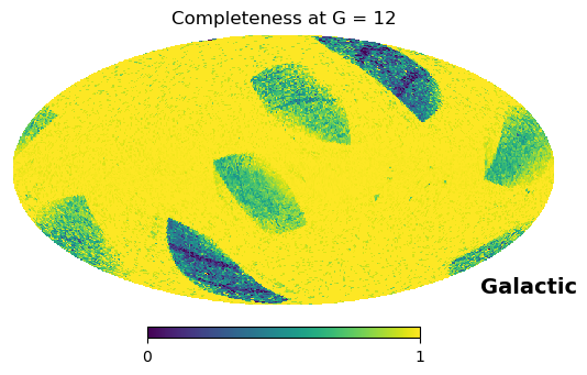
For this plot we visualise the selection function at G=12.

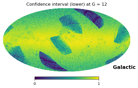
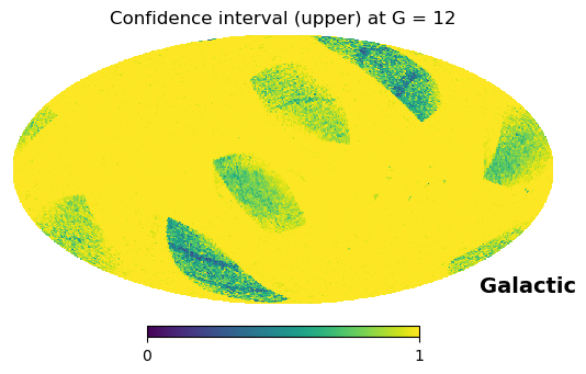
The .query() method returns the posterior probability of a source satisfying the user-defined criteria, along with the associated confidence interval (its lower and upper boundaries), if the user needed it. We visualise both:

# Specify the healpix level
hplevel = 6
# Specify at which magnitude you want to visualise the selection fraction:
G = 12

coords_of_centers = utils.get_healpix_centers(hplevel)
gmag = np.ones_like(coords_of_centers) * G

# The `query` interface is completely resembles the one in the `SubsampleSelectionFunction` class,
# except the `return_confidence` parameter, replacing the parameter `return_variance` in the former implementation
p, ci_lo, ci_hi \
    = subsampleSF_HMLE.query(coords_of_centers, hplevel=hplevel, phot_g_mean_mag_=gmag, return_confidence=True)

plt.figure()
hp.mollview(p, hold=True, min=0, max=1, title="Completeness at G = {}".format(G), coord='CG')
plt.show()
plt.close()

plt.figure()
hp.mollview(ci_lo, hold=True, min=0, max=1, title="Confidence interval (lower) at G = {}".format(G), coord='CG')
plt.show()
plt.close()

plt.figure()
hp.mollview(ci_hi, hold=True, min=0, max=1, title="Confidence interval (upper) at G = {}".format(G), coord='CG')
plt.show()
plt.close()

Use case 2 - first SubsampleSelectionFunction, then apply HMLE

Here, we fetch the same data with the SubsampleSelectionFunction class, then pass it to the new class. Estimate the confidence interval at the 68% C.L.

%%time
subsampleSF \
    = subsample.SubsampleSelectionFunction(subsample_query='has_xp_continuous', \
                                           file_name='dr3_xp_hpx6', hplevel_and_binning=inDict)

subsampleSF_HMLE = subsample.SubsampleSelectionFunctionHMLE().use(subsampleSF, z=0.99)

/Users/cantat/gaiaunlimited/evgeny/gaiaunlimited/src/gaiaunlimited/selectionfunctions/subsample.py:29: FutureWarning: The return type of `Dataset.dims` will be changed to return a set of dimension names in future, in order to be more consistent with `DataArray.dims`. To access a mapping from dimension names to lengths, please use `Dataset.sizes`.
  if ds.dims.keys() - set(["ipix"]) == {"g", "c"}:
/Users/cantat/gaiaunlimited/evgeny/gaiaunlimited/src/gaiaunlimited/selectionfunctions/subsample.py:32: FutureWarning: The return type of `Dataset.dims` will be changed to return a set of dimension names in future, in order to be more consistent with `DataArray.dims`. To access a mapping from dimension names to lengths, please use `Dataset.sizes`.
  diff = set(ds["logitp"].dims) - ds.dims.keys()

CPU times: user 610 ms, sys: 162 ms, total: 772 ms
Wall time: 771 ms

Let us dive into the internals of the SubsampleSelectionFunctionHMLE class. We can extract more interesting information using them.

The main product of the HMLE algorithm is the hds list. The l-th element of this list corresponds to the l-th level of the healpix hierarchy. Each element is a dataset (xarray.Dataset) that contains: the number of stars in the parent catalogue 'n', number of stars in the subsample 'k', logit of the probability of completeness 'logitp', and the boundaries of the confidence intervals 'ci_lo' and 'ci_hi' (if the confidence level z was provided before). These distributions are defined on the same healpixels (zeroth dimension) vs. magnitudes vs. whatever was requested (first and subsequent dimensions) grid.

# Plot the sky maps off the `hds` list

hplevel = 6

# Collect the total number of sources inside every healpix, _regardless their magnitudes_ (the summation over the last axis is for that)
n = subsampleSF_HMLE.hds[hplevel]['n'].sum(axis=-1)
k = subsampleSF_HMLE.hds[hplevel]['k'].sum(axis=-1)

# We need to do this in order to harmonize the healpix enumeration scheme
ipix = utils.coord2healpix(coords_of_centers, 'icrs', nside=hp.order2nside(hplevel), nest=True)
n = n[ipix]
k = k[ipix]

plt.figure()
hp.mollview(k, hold=True, norm='log', cmap='inferno', title="No. stars per healpix that have XP spectrum", coord='CG')
plt.show()
plt.close()

plt.figure()
hp.mollview(k/n, hold=True, cmap='inferno', title="Maximum likelihood estimate for the completeness of subsample", coord='CG')
plt.show()
plt.close()

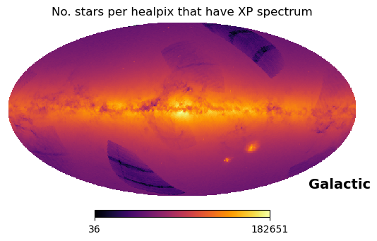
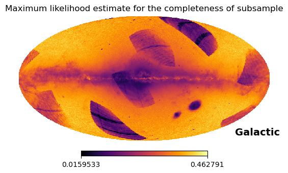
The integral distribution of the number of sources (i.e. summed up by the magnitudes) have no empty healpixels (but does at higher HEALPix levels), so using the MLE as completeness estimate is fine. On the contrary, the distribution over the magnitudes have some empty bins at the highest and lowest values.

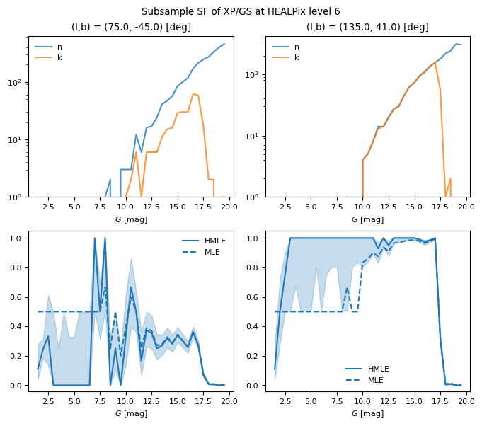
To see this, let us pick two directions on the sky: a poor pixel and a rich pixel.

from scipy.special import expit, logit
from astropy_healpix import HEALPix
from astropy.coordinates import SkyCoord
import matplotlib.pyplot as plt


plt.rc('font', size=8.0)
inch = 2.54  ## cm
width, height = 17/inch, 15/inch
plt.figure(figsize=(width, height), layout='constrained')
plt.suptitle(f"Subsample SF of XP/GS at HEALPix level {hplevel}")

prop_cycle = plt.rcParams['axes.prop_cycle']
colors = prop_cycle.by_key()['color']

l = [ 75, 135]
b = [-45,  41]
co = SkyCoord(l, b, frame='galactic', unit='deg')
healpix = HEALPix(nside=hp.order2nside(hplevel), order='nested', frame='icrs')
ipix = healpix.skycoord_to_healpix(co)
print("ipix:", ipix)

# The MLE Dataset
ds0 = subsampleSF.ds
# Augment the non-observed data with the non-informed estimate
p0 = expit(ds0['logitp'].fillna(logit(0.5)))
# NB: The MLE data is always at the highest healpix level,
# the one that was requested with the constructor of the `SubsampleSelectionFunction` class

# The HMLE Dataset at the required healpix level
# This dataset has the same structure as the MLE dataset, except the 'ci_lo' and 'ci_hi' fields
ds = subsampleSF_HMLE.hds[hplevel]
G = ds['phot_g_mean_mag_']
n = ds['n']
k = ds['k']
p = expit(ds['logitp'])
ci_lo = ds['ci_lo']
ci_hi = ds['ci_hi']

for i, hpx in enumerate(ipix):
    plt.subplot(2, 2, 1+i)
    plt.title(f"(l,b) = ({co[i].l.deg}, {co[i].b.deg}) [deg]")
    plt.plot(G, n[hpx], color=colors[0], alpha=0.8, label="n")
    plt.plot(G, k[hpx], color=colors[1], alpha=0.8, label="k")
    plt.legend(frameon=False)
    plt.xlabel("$G$ [mag]")
    plt.yscale('log')
    plt.ylim(ymin=1)

    plt.subplot(2, 2, 2+1+i)
    plt.plot(G, p[hpx], color=colors[0], label="HMLE")
    plt.plot(G, p0[hpx], '--', color=colors[0], label="MLE")
    plt.fill_between(G, ci_lo[hpx], ci_hi[hpx], color=colors[0], alpha=0.25)
    plt.legend(frameon=False)
    plt.xlabel("$G$ [mag]")
    plt.ylim(ymin=-0.04)

#plt.savefig(f"dr3_xp_hpx{hplevel}_twopix.pdf")
plt.show()
plt.close()

ipix: [19229  7654]

Use case 2B - apply HMLE to your own data

This example is the exact same as Case 2 above (we fetched the data with the SubsampleSelectionFunction module), but here we pass it to the HMLE module as a xarray.Dataset. When you do this, you also need to explicitly provide the dictionary describing the binning (in healpix, in magnitude, etc).

The binning data can also be passed as a pandas.DataFrame.

subsampleSF \
    = subsample.SubsampleSelectionFunction(subsample_query='has_xp_continuous', \
                                           file_name='dr3_xp_hpx6', hplevel_and_binning=inDict)

subsampleSF_HMLE = subsample.SubsampleSelectionFunctionHMLE().use(subsampleSF.ds, inDict, z=0.99)

/Users/cantat/gaiaunlimited/evgeny/gaiaunlimited/src/gaiaunlimited/selectionfunctions/subsample.py:29: FutureWarning: The return type of `Dataset.dims` will be changed to return a set of dimension names in future, in order to be more consistent with `DataArray.dims`. To access a mapping from dimension names to lengths, please use `Dataset.sizes`.
  if ds.dims.keys() - set(["ipix"]) == {"g", "c"}:
/Users/cantat/gaiaunlimited/evgeny/gaiaunlimited/src/gaiaunlimited/selectionfunctions/subsample.py:32: FutureWarning: The return type of `Dataset.dims` will be changed to return a set of dimension names in future, in order to be more consistent with `DataArray.dims`. To access a mapping from dimension names to lengths, please use `Dataset.sizes`.
  diff = set(ds["logitp"].dims) - ds.dims.keys()